Hipparchos, 2014
Orbital Evolution in Extra-solar systems
George Voyatzis
Section of Astronomy, Astrophysics and
Mechanics, Department of Physics, Aristotle University of Thessaloniki, Greece.
Abstract
Nowadays, extra-solar systems are a hot research topic including
various aspects, as observation, formation, composition etc. In this paper, we
present the main orbital and dynamical features of these systems and discuss
the evolution of planetary orbits in multi-planet systems. Particularly, we
consider the dynamics of a two-planet system modeled by the general three body
problem. Complicated orbits and chaos due to the mutual planetary interactions
occur. However, regions of regular orbits in phase space can host planetary
systems with long-term stability.
1. Introduction
After
the detection of the first three planets orbiting the pulsar PSR B1257+12 in 1992 and the first
planet orbiting the main-sequence star 51
Pegasi in 1996, a significant growth of detected exoplanets took place,
which currently seems to be
rather exponential. One of the most reliable catalogs of exoplanets is given by
the Extrasolar Planets Encyclopedia
(EPE) [1]. Very recently, on 6th
March 2014, a set of 702 new planet candidates, observed by the Kepler Space
Telescope (KST), were added in
this catalog, which now includes 1778 planets arranged in 1099 planetary systems[1].
In the blue histogram of figure 1, we present how the number of discovered
exoplanets increases year by year and in the red one how the planets are
distributed in the planetary systems. A number of 637 systems contains only one
planet, while the rest 1141 planets are arranged in 462 multi-planet systems
most of them consisting of two planets. The most “populated” system is Kepler-90 (around the star KOI-351), which seems to consist of
seven planets[2].
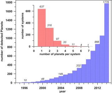
Figure 1. The blue histogram shows how many exoplanets
have been discovered until the indicated year. The abrupt increase of the
number in 2014 (although this number refers to March, 6th) is due to
the addition of a set of 702 planets discovered by the KST. The red histogram
shows how the 1778 planets are arranged in the 1099 planetary systems.
The
first detection method used was the method of radial velocity or Doppler
method and most of the known exoplanets have been discovered by this
method, which is still widely used. The transit
method has also been proved
efficient, mainly after its application by the KST. Gravitational microlencing, reflection/emission methods,
polarimetry e.t.c. can also be
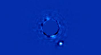
used as detection methods [2]. Direct
imaging has given few yet
spectacular results, firstly,
with the discovery of the planet Formalhaut
b by the Hubble telescope and, recently with the discovery of Beta Pictoris b by the Gemini Planet
Imager (see figure 2). The region of observations has a radius of about 103
l.y. and it is estimated that our galaxy contains 400 billion planets. The
closest exoplanet to our Solar system is the Epsilon Eridani b in a distance of 10 l.y..
Most
exoplanets are classified as hot Jupiters,
namely gas giant planets that
are very close to their host star, e.g. HD
102956 b which has mass equal to Jupiter’s mass (1MJ), semimajor axis 0.08AU and period 6,5 days. Very massive
planets have been found, either close to their host star (e.g. Kepler-39 b with mass 20MJ, semimajor axis 0.15 AU
and period 21 days), or very far from their host star (e.g. HIP 78530 b has mass 24MJ, semimajor axis 710AU and period 12Ky). As detection techniques are improved, smaller planets are
detected. Many of them have masses equal to 10-20 times the mass of the Earth, are possibly gaseous and are
called Mini-Neptunes. Nevertheless,
planets with mass of the order of the Earth's
and of similar radius can be detected by the KST. They are possibly
terrestrial (rocky) planets and become
very interesting for detailed study, when they are located in a habitable zone,
e.g. the Gliese 667C c [3].
Studying
the general structure of the known extrasolar systems we can certainly argue
that our Solar system is an exception. Thus, the proposed mechanisms for
formation and evolution of planetary systems should be revised and generalized.
In the following, we focus on the orbital characteristics of multi-planet systems, the conditions required for their long-term stability and the role of planetary
resonance.
2. Orbital and dynamical features
Considering
a system consisting of a star and a planet (assumed as point masses) we expect
Keplerian elliptic planetary orbits around the star with period T, semi-major axis a, eccentricity e and
inclination I. From the observations
and after applying particular fitting methods (see e.g. [2]) these orbital
parameters can be estimated approximately for each observed planet. In figure
3, we plot the distributions a-e and T-e of 623 planets for which we have an estimation of the orbital
parameters in the list of EPE. The fact that the majority of planets appears
with small semi-major axes and periods is possibly caused by an observational
selection bias, since large and close to the star planets are more easily
detectable. Most of these close-to-star planets have also small orbital eccentricities possibly caused by tidal
circulation [4].
An important orbital feature that is
clearly seen from the plot of figure 3 is that we obtain the existene of many
planets with large eccentricities. E.g. an extreme planet is HD 20782 b with a=1.38AU and e=0.97. High eccentric orbits are also
observed in multi-planet systems. E.g. in the two-planet system around the star
HD 7449 the inner and the outer
planets have eccentricity 0.82 and 0.53, respectively (see figure 4). The
formation of such highly eccentric planetary systems is not sufficiently
supported by the current theories. However, long-term evolution stability is
possible and can be proved as we explain in the last section.
Figure 3. The distribution of exoplanets in the planes a-e (blue dots) and T-e (red crosses). Most of the planets have small semi-major axis
(or period) and small eccentricity. There are few more planets, which are
located outside the axis’ limits of
the plot and they are not shown.
Figure 4. The
orbits of the giant planets around the star HD 7449. The eccentricities of the
inner and the outer planet are 0.82 and 0.53, respectively. The semimajor axes
are 2.3AU and 4.96AU, respectively.
The
inclination Io of the
orbital plane with respect to the observer is defined as the angle between the
normal to the planet's orbital plane and the line of the observer to the
star. Most observational methods, and
mainly the transiting method, can observe planets only with inclinations Io»90o.
For radial-velocity observations the inclination is very important for the
computation of the planetary mass because the particular measurements provide
us with an estimation of the quantity m×sin
Io.
The
inclination I defined between the
normal of the orbital plane and the stellar rotational axis is the most
important from a dynamical point of view. In this sense, particular studies
indicate that most planetary systems are inclined [5]. Cases where I»180o,
i.e. planets moving around the star in a direction opposite to
the spin of the star, have also
been indicated in observations making the puzzle of planetary formation quite
complicated. Generally, it seems that in multi-planet systems, planets are
almost co-planar, i.e. the mutual
inclination DI=I1–I2
between two planets is close to zero. However, cases of
high mutual inclination between planets have also been observed, e.g. the planets c and d around Upsilon Andromeda seem to have mutual
inclination larger than 30o.
Mean
motion resonances (MMR) in multi-planet systems appear frequently. Two planets
(1 and 2) are in a MMR, when the
ratio r=T1/T2 of their orbital period is close to a ratio r=p/q of two (small) integers. Computing the
ratio r
of all planet pairs appearing in the multi-planet systems of the EPE list we
obtain a significant number of resonant pairs.
Certainly this number depends on the divergence d=(r-r)/r that we set as a threshold. For divergence
less than 5%, 2% or 1% we find respectively 419, 174 or 83 resonant planetary
pairs. Their distribution to each value r
is shown in figure 5.
Figure 5. The distribution of resonant planetary pairs
at each resonance p/q. Different color bars correspond to different threshold
values of the difference of the ratio T1/T2 from the ratio p/q. For each pair we have set as T1 the greater orbital
period.
3. The three body model and orbital evolution
A
two-planet system can be modeled by a system of three point masses m0, m1 and m2
representing the star, the inner and the outer planet, respectively. Thus m0>>m1,2 and initially it holds a1<a2 . Although the planetary masses are very small, the
mutual planetary interaction is not negligible if we want to study the orbital
evolution for moderate or long time intervals and during such an evolution the inner planet may
become outer and vice versa.
Let Xi
be the position vector of the three bodies in an inertial frame. Following Poincaré, we can consider for the planets the astrocentric
position vectors ri=Xi-X0
and the barycentric momenta pi=mi(dXi/dt) and
write the Hamiltonian of the system in the form H=H0+H1
, where
and
![]()
The term H0 describes the evolution
of the planets in the framework of the two body problem (unperturbed
star-planet system). The second term
includes the planetary interactions and is a perturbation term for the
integrable part H0. Subsequently, we have a nonintegrable model
of 6 degrees of freedom and the corresponding canonical equations of motion are
integrated numerically. In this system we have the conservation of energy and
the three components of the angular momentum vector [6].
A second formalism for the planetary
three-body model results if we express the Hamiltonian in orbital elements[3]
![]()
where wi is the argument of periastron, Wi is the
longitude of ascending node and li is the mean longitude (index
i=1,2 refers to the particular
planet) [7]. From the above Hamiltonian simplified models can be constructed by
the method of averaging.
By averaging that fast motion on the ellipse, given by
the angles li, we obtain the secular model. Up to second order in
masses we obtain that the phase space structure depends on the planetary mass
ratio m1/m2. Also, it turns out that the semimajor axes
remain almost constant and in a coplanar system the eccentricities e1
and e2 oscillate slowly with opposite phases. Actually, in a 3D system the conservation of
angular momentum is expressed as
![]()
where aι are almost constants, which depend on the masses and semimajor axes of the planets. Another feature of secular
dynamics is also the libration of the difference Dv=v2-v1 of the
longitude of pericenter of the two planets [8].
When the system is close to a MMR,
the averaging should exclude slow “angle combinations” [7][8]. For a resonance r=p/q we can define the resonant (slow)
angles si=
ql1-pl2+(p-q)vi.
If s1
or s2
librates we argue that the planetary system involves inside the resonance. The
center of a resonant domain or the “exact resonance” is given by the stable
stationary solutions i.e. the minima of the averaged Hamiltonian where si=const.
In resonant evolution, the semimajor axes are not invariant (as in the secular
evolution), but we can derive the constraint![]() , where bI are almost constants and depend on the masses and the
resonance.
, where bI are almost constants and depend on the masses and the
resonance.
The
conservation of the angular momentum can be used for reducing further the
degrees of freedom by two. This is achieved by choosing a suitable rotating frame Oxyz, where the star and
one of the planets (say planet 1) are
always located on the plane Oxz
and Oz axis is chosen to coincide
with the vector of angular momentum. In this rotating frame, the planet 2 is
given by the components (x,y,z)=(x2,y2,z2)
,but only the component c=x1
is required for the determination of the planet 1. Thus the system is described
by four degrees of freedom and
Hamiltonian
![]()
where pc, px, py and pz
are the conjugate momenta [9]. In this formalism, we can obtain directly the
well known circular restricted three body problem, if we set m2=0, c=const. and n=const., where n is the angular velocity of the rotating frame.
Hamiltonian,
H, written for the rotating frame is
convenient, when we want to study the dynamics through the periodic orbits of
the system. The families of periodic orbits of the restricted three body
problem, generally, are continued to the general three body problem and can be
computed in a systematic way [10][9]. Periodic orbits are associated with the
stationary solutions of the approximate averaged Hamiltonian mentioned above.
Families of periodic orbits are either “circular” or “elliptic”. Along a
circular family the ratio r=T2/T1 of planetary periods varies.
Families of elliptic orbits bifurcate
from the circular family, when r=p/q (i.e. at resonances). Along these
bifurcating families r remains almost constant. Thus, all elliptic
periodic orbits are resonant and, actually, present the “exact” dynamical resonance
[11]. Linear stability analysis can be performed classifying the periodic
orbits as stable or unstable.
4. Orbital Evolution of HD 82943b,c
In this section, we present an example of the dynamical analysis of the
orbital evolution of the extra-solar
system around the star HD 82943 (with mass 1.18MSun). Three
planets have been discovered for this star, the planets b,c and d with period
442, 219 and 1078 days, respectively. The first two planets have masses ~4.8MJ and the third one is quite
smaller with mass 0.29MJ.
So, we can neglect the interaction of the third planet to the other two heavy
planets and study the evolution in the framework of the three body model with
inner planet (P1) the planet c and outer planet (P2) the
planet b. The orbital parameters are the following
|
|
m (MJ) |
a (AU) |
e |
v (o) |
|
P1 |
4.78 |
0.75 |
0.425 |
133 |
|
P2 |
4.80 |
1.20 |
0.203 |
107 |
No
estimation is given for the position of the planets in their elliptic orbits. The two planets are
coplanar with I0=19o.
Also the system is resonant with T2/T1»2.0.
For
the planetary ratio m2/m1»1 and for
the region of the given eccentricity values, we find that there exists a family of periodic orbits,
which is symmetric and corresponds to
a planetary configuration with aligned planets, i.e. Dv=0o,
and when the inner planet is at periastron the outer planet could be found at
apoastron, i.e. s1=0o.
Thus, we will consider for our analysis two planetary initial configurations: configuration A with Dv=0o
and configuration B with Dv=-26o
(the value given in the list). We consider that P1 is initially
located at periastron and P2 at apoastron[4].
In
Figure 6, we present the evolution of the eccentricities and the apsidal
difference Dv
for configurations A and B. When the planets are aligned (configuration A) the
system evolves regularly, Dv
librates indicating the resonant evolution and the eccentricities show small (anti-phase) oscillations.
However, if we consider the configuration B, we see that Dv
rotates. Although, the evolution initially seems regular, after 1.2Ky the system is destabilized. Small
planetary encounters occur and the outer planet increases its eccentricity to values almost up to 1 (collision
with the star).
Figure 6. The
evolution of planets c (P1) and b (P2) of the system HD
82943 for the two different initial configurations A and B
(see the text). In the left panels, the time evolution of the
eccentricities and the planetary apsidal difference is presented. In the
middle, we show the initial configuration of the system and the orbit in its
first moments of evolution. In the right, the planetary orbits at about 1.5Ky are
shown. The destabilization in the configuration B is obvious.
In
order to understand the underlying dynamics of the above evolution, we depict
the qualitative type of evolution of all orbits in particular domains of the
phase space by constructing dynamical
maps of stability, namely we consider plane grids of initial conditions and
for each grid point we evolve the orbits and classify them as regular or
chaotic by computing a chaoticity index e.g. the DFLI in our case [12]. In the maps presented below, light (yellow)
colors indicate chaotic motion while dark ones (blue-green) corresponds to
regular evolution.
Figure 7.
Dynamical maps of stability for the system HD 82943. a) map in the plane of
initial eccentricities for the configuration A, b) map in the plane of initial
eccentricities for the configuration B, c) map in the plane of initial resonant
angles (s1,Dv) at (e1,e2)=(0.425, 0.16). Yellow regions indicate chaos while
dark colors correspond to regular orbits. The star shows the starting point of
the system.
In
panels (a) and (b) of figure 7, we consider all possible eccentricities of the
two planets (keeping the rest orbital parameters as it is defined in the two
configurations A and B, respectively). We obtain that in configuration A (panel
a) there is a strip of regular orbits. The backbone of this region is the
stable 2:1 resonant family of periodic orbits for the particular planetary
masses (the gray characteristic curve). If we project the planetary evolution
in the plane of eccentricities, we obtain oscillations centered at the
eccentricity values of a periodic orbit at about (e1,e2)=(0.42,
0.16). When the planets are not
initially set to be aligned (Dv¹0o),
the regions of regular orbits in the dynamical stability maps shrink and show a
shift from the characteristic curve of periodic orbits. Subsequently, for Dv=-26o
the system seems to be located in the chaotic region (but close to the regular
one). Thus, the system destabilizes and shows diffusion in the wide chaotic sea
of the phase space, where the evolution is strongly irregular. In these
dynamical regions, the system suffers from close encounters, which possibly
lead one of the planets to a collision with a star or to escape or to a
planet-planet collision.
In
panel (c) of figure 7, we consider the eccentricity values (0.42, 0.16),
mentioned above, and construct a dynamical map for a grid of initial conditions
with all possible planetary alignments Dv and initial
angle positions (presented by the resonant angle s1).
The central regular region is associated with the periodic orbit, located in
this map at (0,0). Again, we see that the configuration B locates the system in
the chaotic region. We may conclude from the above analysis that the orbital
parameters given in the EPE list should be revised. Namely, stability is
guaranteed for |Dv|<26o.
Also, if we assume slightly smaller planetary masses, then the regular region
is expanded and the system can be located in the regular region. Possible
planetary mutual inclination may also
be a stabilization factor.
When two
planets have large enough eccentricities,
then planetary close encounters (and subsequently destabilization) are,
generally, unavoidable unless
the system is in resonance. Resonances can offer a phase protection, i.e.
although orbits are close (or intersect), the planets cannot be found close to
each other. It has been shown that stable resonant periodic orbits can exist
for very large eccentricities and therefore, regions of stability can be
located. However, as eccentricities increase, the stability domain around the central periodic orbit
shrinks. Thus, a real planetary system
with large eccentricities may be found only very close to a stable resonant
periodic orbit. This, for example, should be the case for the system HD 7449
presented in figure 4.
References
[1] F. Roques and J. Schneider, The Extrasolar
Planets Encyclopedia, http://exoplanet.eu
[2] Cassen P., Guillot T. and Quirrenbach A.,
Extrasolar Planets, Springer, 2006.
[3] Planetary Habitability Laboratory,
University of Puerto Rico, http://phl.upr.edu/hec.
[4] Sun Y.S, Ferraz-Mello S., Zhou J.L.,
Exoplanets: Detection, Formation and Dynamics, Cambridge University Press, 2008
[5] Atkinson N, Most Exoplanetary Solar Systems
Have Inclined Orbits, http://www.universetoday.com/82601/
[6] Beauge C., S. Ferraz-Mello, T. Michtchenko,
in Extrasolar Planets, edited by R. Dvorak, Wiley-Vch, 2008
[7] Murray C.D. and Dermott S.F., Solar system
dynamics, Cambridge University Press, 1999
[8] T. Michtchenko, S. Ferraz-Mello, Beauge C.,
in Extrasolar Planets, edited by R. Dvorak, Wiley-Vch, 2008
[9] Antoniadou, K.I., Voyatzis, G, 2/1 resonant
periodic orbits in three dimensional planetary systems, CMDA, 115, 161, 2013.
[10] G. Voyatzis, T. Kotoulas, and J. D.
Hadjidemetriou, On the 2/1 resonant planetary dynamics - periodic orbits and
dynamical stability. MNRAS, 395, 2147, 2009.
[11] Hadjidemetriou J., Symmetric and asymmetric
librations in extrasolar planetary
systems: a global view. CMDA, 95, 225, 2006.
[12] Voyatzis, G.: Chaos, order, and periodic
orbits in 3:1 resonant planetary dynamics. Astrophys. J. 675, 802, 2008.